
What an AI implementation looks like, by sector.
For each discipline we show how we approach an AI implementation: the work process, the choices and the result we steer on. Concrete, within your standards, with the human who decides and signs.
No promised percentages, but the method, the scientific reasoning behind it and exactly how we settle the result against your own baseline measurement.
These scenarios are illustrative and based on typical work processes in the sector, not the names of existing clients.
 01Logistics & transport
Dynamic route optimisation inside a 3PL with daily plan cycle.
What a VRP approach with live traffic and EU driving-time rules looks like for a mid-size 3PL. The model proposes options, the planner keeps the final call.
- Approach
- The daily runs are modelled as a capacitated VRP with time windows (CVRPTW): a time window per order, a load capacity per vehicle. A metaheuristic (guided local search / ALNS) finds a strongly improved plan within seconds, shown next to the planner's own version.
- Reasoning
- The VRP is NP-hard: solving it exactly is infeasible at hundreds of stops, so heuristics that provably come close to optimal. Travel times are time-dependent (peak ≠ off-peak) and the EU driving-time rules, Regulation (EC) 561/2006 (max 9h driving, break after 4.5h, 11h daily rest), sit in the model as a hard constraint, not an after-the-fact check.
- How we measure
- Measured against your planning today: kilometres, runs and promised-vs-met time windows (OTD). We calibrate on historical days first, before a single run goes live.
- What we need
- Order history with addresses and time windows, vehicle and driver capacity, and today's OTD figures as a baseline.
- CVRPTW
- Regulation (EC) 561/2006
- TMS-IFTMIN
- OTD baseline
 02Food manufacturing
Predictive maintenance on a packaging or grading line, with an audit-ready record.
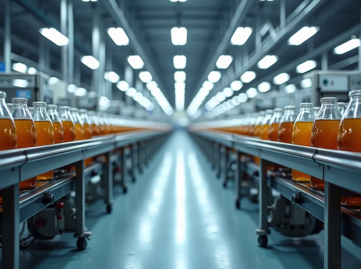
How a sensor stream (vibration, temperature, cycle time) on a packaging or grading line in a cold-chain environment is set up, without interrupting production.
- Approach
- Vibration, temperature and cycle-time sensors on the critical drives. From the vibration signal the bearing defect frequencies (BPFO/BPFI, depending on bearing geometry and RPM) are tracked via envelope analysis, demodulation around the bearing resonance; a rising trend schedules the CMMS work order into the planned change-over, not during the run.
- Reasoning
- Early bearing wear shows up as energy at specific defect frequencies and as rising kurtosis/RMS velocity (cf. the vibration classes in ISO 20816, successor to ISO 10816), often weeks before audible failure. Maintenance is a prerequisite programme (PRP) under FSSC 22000, not a CCP; the same sensor and logging backbone does capture the cold-chain CCP (product temperature) in a hash-chained audit trail.
- How we measure
- Unplanned downtime and overrun per line, set against your maintenance history. We watch the false-alarm rate explicitly: a predictor that cries wolf too often costs change-over time and trust.
- What we need
- Access to existing PLC/sensor data or a few added vibration sensors, bearing specs and RPMs, and today's downtime records.
- FFT bearing analysis
- PRP maintenance
- Cold-chain CCP
- Hash-chained audit trail
 03Agri-food & greenhouse
Yield forecast and labour planning inside a tomato greenhouse.
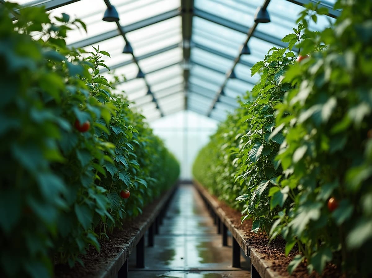
How a 7-day yield forecast per greenhouse bay is built from climate data and historical pick data, to drive the pick-crew schedule.
- Approach
- A statistical model forecasts the pickable kilos per bay for the next seven days from the PAR light sum, CO₂, 24-hour temperature and EC, calibrated on your own historical pick weights. The forecast feeds the crew schedule directly: how many pick hours, which day, per bay.
- Reasoning
- Tomato yield is strongly driven by intercepted PAR light sum (DLI, mol/m²/day): more light gives more assimilates and fruit weight, with a lag of weeks between flowering and harvest. The 24-hour mean temperature sets the development rate (truss appearance follows degree-days); CO₂ and EC steer photosynthesis and fruit quality.
- How we measure
- Forecast vs. actual picked kilos per bay per day; we report the deviation honestly and adjust. The goal is calmer labour planning, not a perfect forecast.
- What we need
- Climate-computer export (PAR/CO₂/temperature/EC), historical pick records per bay, and the current way of scheduling crews as a comparison.
- PAR light sum / DLI
- Degree-days
- Pick labour
- GlobalG.A.P.
Curious what this means for your organisation?
Start with the free Practice Scan or book an introductory conversation to discuss your situation.